Part 2 of 3. Part 1 set six requirements and showed that only a per-tenant resource with its own ARN satisfies them. This part is the money: why nobody built that design, the S3 Vectors pricing model in detail, a reproducible worked example, and where the break-even sits. Part 3 is the pipeline with code.
Provisioned Stores: The Bill is the Box
On every provisioned vector store — pgvector on RDS/Aurora, OpenSearch domains, self-hosted Qdrant, Milvus or Weaviate, Pinecone pods — the approximate-nearest-neighbour index lives in memory, and memory comes as an instance. You size the instance for your busiest tenant and your busiest minute, then pay for it every hour, busy or idle.
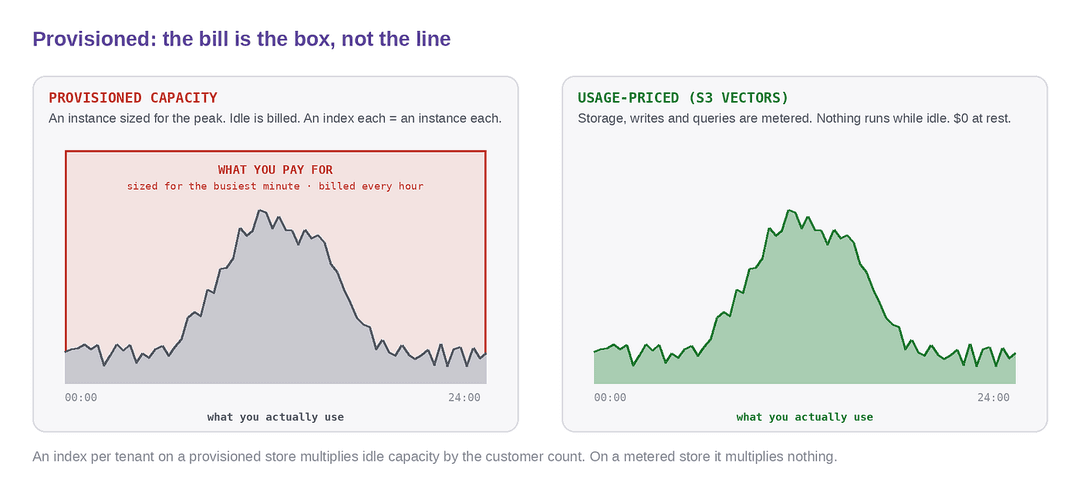
Apply that to “an index per tenant”. An index each means an instance each. As an order of magnitude, an Aurora instance in the smallest useful classes runs from tens to a few hundred dollars a month at list; multiply by a few hundred tenants and the vector layer alone is in the tens of thousands per month before a single query. Add operations: hundreds of clusters to patch, back up, upgrade and monitor.
So teams put everyone in one index and add a filter.
The three workarounds, and the specific thing each one lacks:
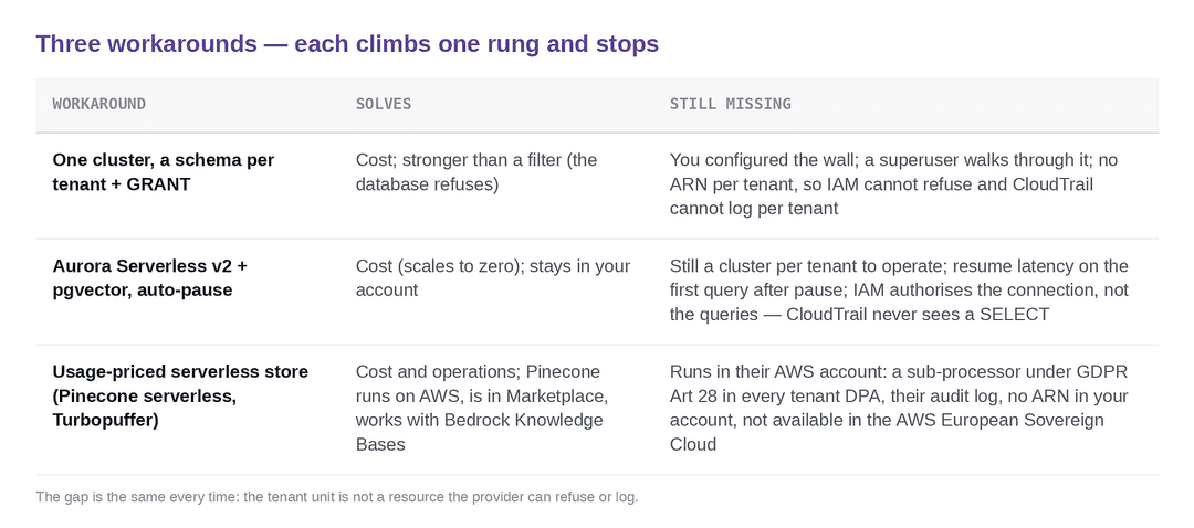
Each climbs one rung and stops. The remainder of this article is about the one store where the per-tenant unit is a first-class resource and nothing is provisioned and what that does to the arithmetic.
S3 Vectors: Limits that Matter for the Per-Tenant Design
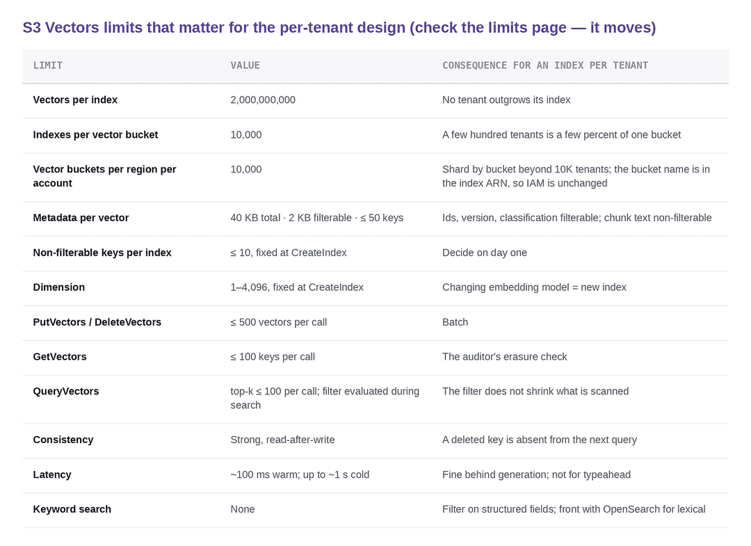
From the limitations page at the time of writing (check it; it moves):
The Pricing Model
Four meters. US East list prices, read September 2026; EU regions run a few percent higher and every ratio below holds. Query pricing was reduced in June 2026 .
WRITE   $0.20 / GB uploaded            (vector + key + all metadata; 128 KB minimum per PutVectors call)
STORE   $0.06 / GB-month               (vector + key + all metadata, non-filterable included)
QUERY   $2.50 / million requests
      + $/TB of "data processed" per query, tiered by the size of the index queried:
            first 100,000 vectors     $0.004 / TB
            100,000 – 10,000,000      $0.002 / TB
            above 10,000,000          $0.0004 / TB
        data processed = (vector + key + FILTERABLE metadata) × vectors in the index
        non-filterable metadata is NOT included
      + $0.01 / GB returned            (256 B minimum per result; first 512 KB per query free)
IDLE    $0                             (nothing is provisioned)
Three consequences fall directly out of this.
- The scan term is proportional to the size of the index you query, not the size of your result. A metadata filter shapes the results; it does not shrink the scan. In a shared index every tenant pays to scan every other tenant’s vectors on every query.
- Non-filterable metadata is free to scan. Putting the chunk text there removes it from the query bill entirely while keeping it in the response.
- The tiers are per index. The first 100K vectors of each index are billed at the top rate. Two 100K indexes cost more to scan than one 200K index.
One trap: AWS bills in binary units. The worked example on the pricing page reproduces only with 1 KB = 1024 B. Here is the check:
KB, GB, TB = 1024, 1024**3, 1024**4
# AWS example: 100,000 vectors × 5.17 KB at $0.004/TB × 1,000,000 queries → they print $1.93
print(round(100_000 * 5.17*KB / TB * 0.004 * 1_000_000, 2))   # 1.93
# AWS example: 6.17 KB × 250,000 vectors × 40 indexes → they print 59 GB
print(round(6.17*KB * 250_000 * 40 / GB, 1))                  # 58.8
Decimal units overstate every byte-based line by 7–10%.
A Reproducible Worked Example
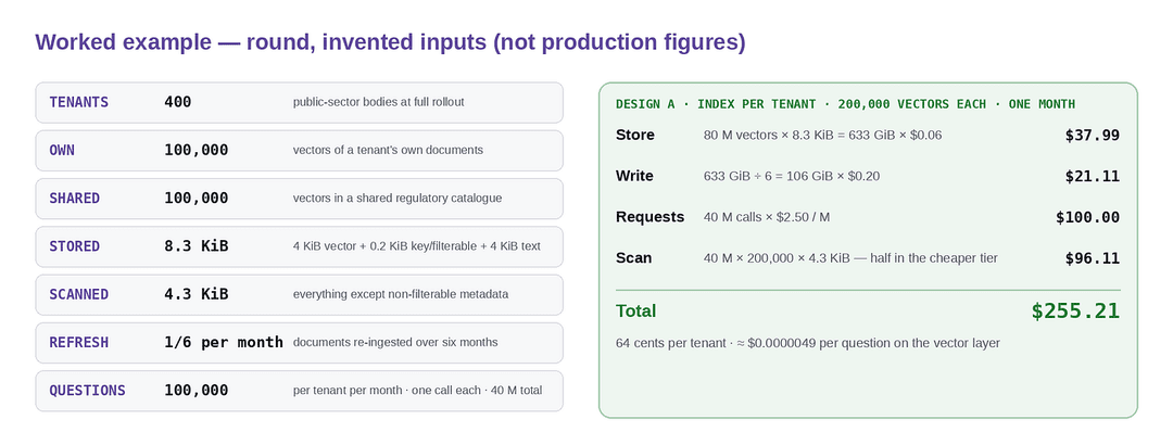
All inputs are round and invented. They are chosen to look like a full rollout of a public-sector SaaS across a few hundred organisations, not to describe any production system.
KB, GB, TB = 1024, 1024**3, 1024**4
TENANTS   = 400          # public-sector bodies at full rollout
OWN       = 100_000      # vectors of a tenant's own documents
SHARED    = 100_000      # vectors in a shared regulatory catalogue (laws, guidance)
STORED_KB = 8.3          # 4 KiB vector + 0.2 KiB key/filterable + 4 KiB chunk_text (non-filterable)
SCANNED_KB= 4.3          # what a query pays for: everything except non-filterable
REFRESH   = 1/6          # fraction of documents re-ingested per month
Q_PER_T   = 100_000      # questions per tenant per month, one QueryVectors each
QUERIES   = TENANTS * Q_PER_T
P_STORE, P_WRITE, P_REQ = 0.06, 0.20, 2.50e-6
def scan_cost(n):                              # $ per query, tiered per index
    b = lambda n: n * SCANNED_KB*KB / TB
    t1 = b(min(n, 100_000))
    t2 = b(max(0, min(n, 10_000_000) - 100_000))
    t3 = b(max(0, n - 10_000_000))
    return t1*0.004 + t2*0.002 + t3*0.0004
def bill(vectors_stored, calls_per_query, scan_per_query):
    gib   = vectors_stored * STORED_KB*KB / GB
    store = gib * P_STORE
    write = gib * REFRESH * P_WRITE
    req   = QUERIES * calls_per_query * P_REQ
    scan  = QUERIES * scan_per_query
    return dict(store=store, write=write, requests=req, scan=scan, total=store+write+req+scan)
Design A — an index per tenant, shared catalogue copied into each index.
Each index holds OWN + SHARED = 200,000 vectors.
A = bill(TENANTS*(OWN+SHARED), 1, scan_cost(OWN+SHARED))
# store 37.99  write 21.11  requests 100.00  scan 96.11  total 255.21
Two hundred and fifty-five dollars a month for four hundred tenants, fully isolated: 64 cents per tenant, at 100,000 questions each. Per question the vector layer is ≈ $0.0000049; the LLM call that answers it is three to four orders of magnitude more.
Design P — one pooled index with a tenant filter.
Everyone’s own vectors plus the catalogue once: 400 × 100,000 + 100,000 = 40,100,000 vectors, and every query scans all of them.
P = bill(TENANTS*OWN + SHARED, 1, scan_cost(TENANTS*OWN + SHARED))
# store 19.04  write 10.58  requests 100.00  scan 5164.44  total 5294.07
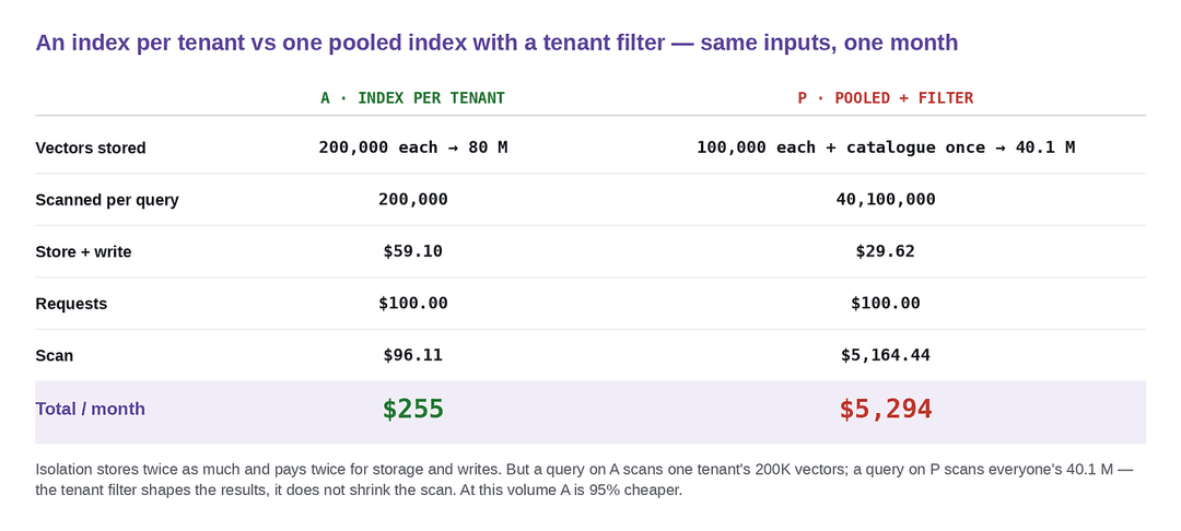
Isolation stores twice as much (the catalogue is duplicated 400×) and pays twice for storage and writes. That is real. But a query on A scans one tenant’s 200K vectors (≈ 840 MiB); a query on P scans 40.1 M (≈ 164 GiB), most of it in the cheapest tier and still ≈ $0.00013 per question. At this volume, A is 95% cheaper.
Where it Crosses
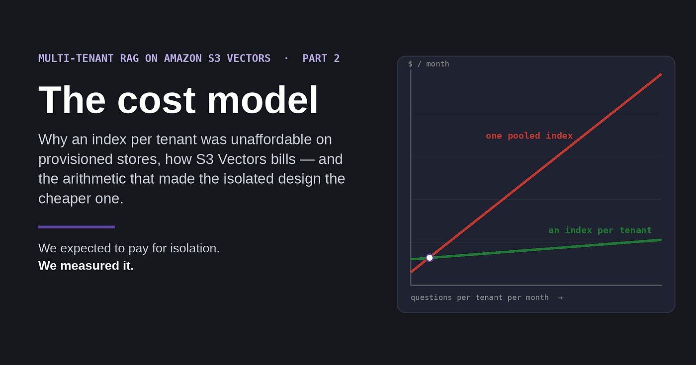
Both designs are linear in query volume: a fixed part (store + write) and a slope (requests + scan). Requests are identical, so:
fixed_gap  = (A['store']+A['write']) - (P['store']+P['write'])        # 29.48  (A pays more)
slope_gap  = scan_cost(TENANTS*OWN+SHARED) - scan_cost(OWN+SHARED)     # per query, P pays more
breakeven  = fixed_gap / slope_gap                                     # ≈ 233,000 queries/month
breakeven / TENANTS                                                    # ≈ 600 per tenant per month
Below about 600 questions per tenant per month, the pooled design is cheaper by at most $29 across all four hundred tenants. Above it, isolation is cheaper, and the gap widens linearly.
It does not widen without bound: because the request fee is the same in both, the ratio of the two bills tends towards (request + P’s scan) ÷ (request + A’s scan) ≈ 27× as volume grows.
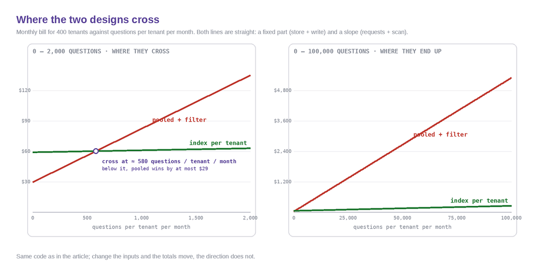
The reason this surprised us: the unit of billing, bytes of the index you touch, rewards exactly the structure that Part 1’s requirements need. Cost and isolation point the same way. Change the inputs and the totals move; the direction does not.
The Day One Decision: Non-Filterable Metadata
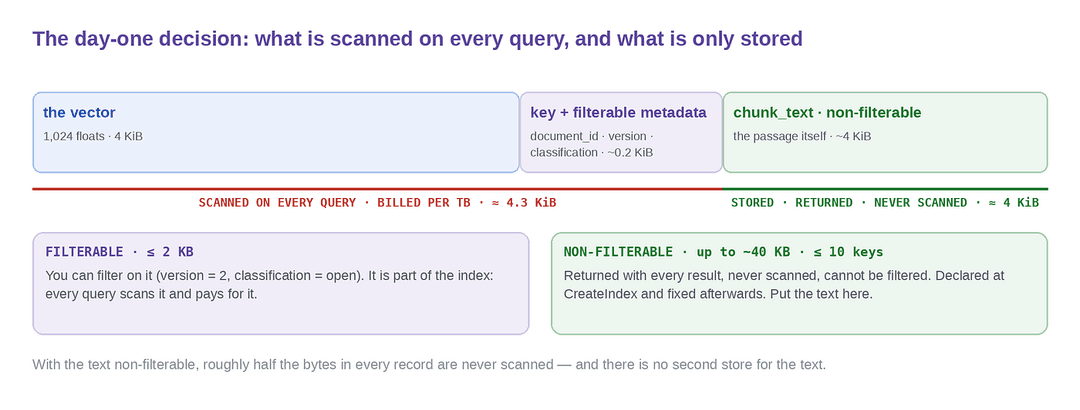
In the record model above, chunk_text (≈ 4 KiB) is non-filterable. If it were filterable it would be scanned on every query, and the per-record scan size would go from 4.3 KiB to 8.3 KiB, roughly doubling the scan line in both designs. It also could not exceed 2 KB. Declaring it non-filterable at CreateIndex keeps it in the index (no second store for text), returns it with every result, and takes it out of the scan.
The constraints: at most 10 non-filterable keys per index, fixed at creation, and non-filterable keys cannot appear in a filter. So anything you filter on -document_id, version, classification — stays filterable and small.
One nuance for the honest version: on a small per-tenant index the request fee is the larger part ($100 vs $96 above), so the non-filterable saving is “half the scanned bytes”, not “half the bill”. On the pooled index, where scan is 98% of query cost, it is close to half the bill.
The Shared Catalogue: Copy into Every Index, or Search Two?
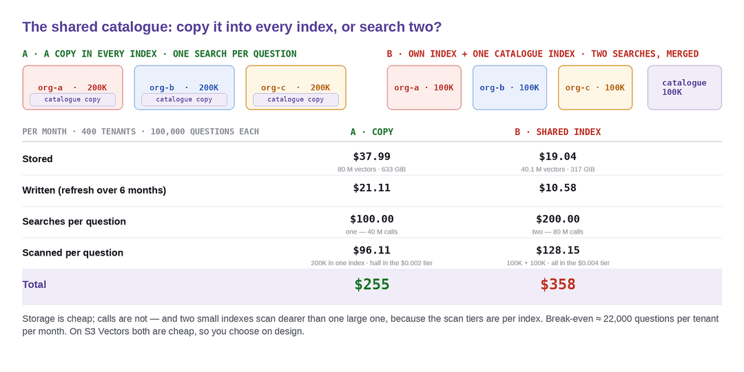
A regulation in the shared catalogue applies to every tenant. Two designs that both satisfy Part 1:
- A — copy it into every tenant’s index. One
QueryVectorsper question; the catalogue's vectors are duplicated per tenant. - B — one shared catalogue index, searched alongside. Two
QueryVectorsper question (own index + catalogue index), results merged in code; catalogue stored once.
A = bill(TENANTS*(OWN+SHARED), 1, scan_cost(OWN+SHARED))                   # 255.21
B = bill(TENANTS*OWN + SHARED, 2, scan_cost(OWN) + scan_cost(SHARED))      # store 19.04 write 10.58 requests 200.00 scan 128.15 total 357.78
B halves storage and writes, then pays twice the request fee — and, less obviously, scans more: two indexes of 100K each stay entirely in the $0.004/TB tier, while A’s single 200K index puts half of every scan in the $0.002/TB tier. Storage is cheap; calls are not; and two small indexes scan dearer than one large one. Break-even is about 22,000 questions per tenant per month; below it B wins by under $30.
The practical point is not which wins. It is that on S3 Vectors both are cheap, so you choose on design: one search, one index, one CloudTrail stream per tenant, no merge code (A) versus one place to update (B). On a provisioned store the copies in A would be hundreds of gigabytes of RAM across many instances and the choice would not exist.
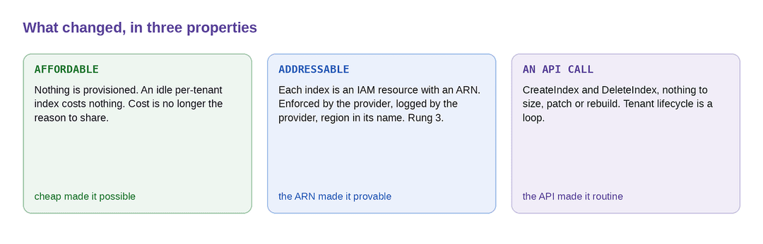
What Changed
Affordable.
Nothing is provisioned. A per-tenant index that is idle costs nothing. Cost is no longer the reason to share.
Addressable.
Each index is an IAM resource with an ARN. The boundary is enforced by the provider, logged by the provider, and carries its region in its name. This is rung 3 from Part 1, and the only one of the three that matters for the requirements table.
An API call.
CreateIndex and DeleteIndex, with nothing to size, patch or rebuild. Tenant lifecycle is a loop.
Part 3 builds it: ingestion with chosen keys, per-request scoped credentials, the deliberate wrong-index test, erasure with GetVectors verification, and CloudTrail data events queried by ARN.
Prices are AWS US East list, September 2026, and change; the code above is the calculation, so re-run it with the current page. All volumes are round, invented inputs stated in the code. No production figures appear in this series.